Week #15

04 Feb 2019

BMCC dataset QuickNAT overfitting

View codes on Github Compare to Unet, the result of QuickNAT has less noise.

QuickNAT	Unet	Groundtruth

Figure 1. Result Comparison of Unet and QuickNAT on BMCC dataset overfitting

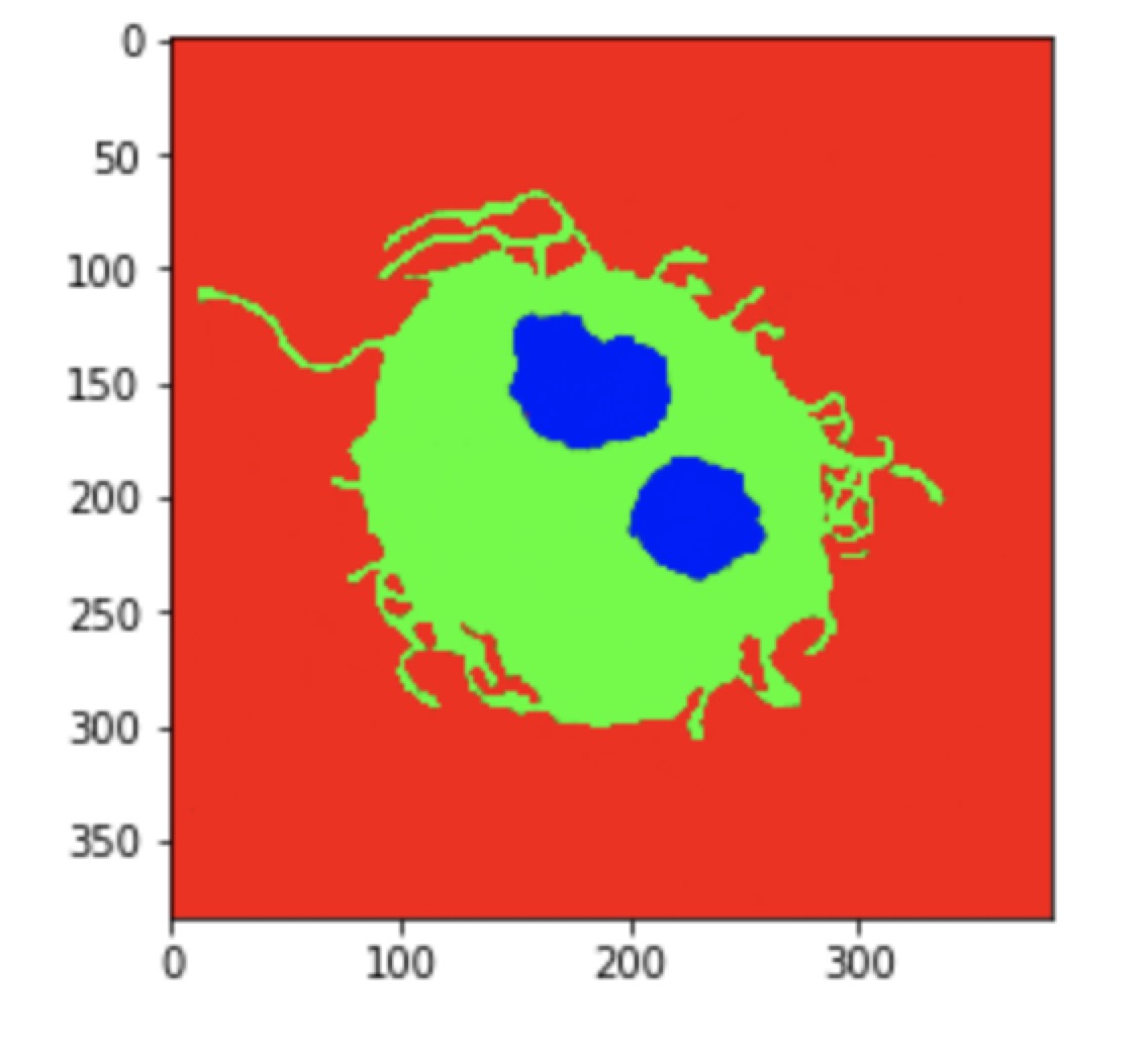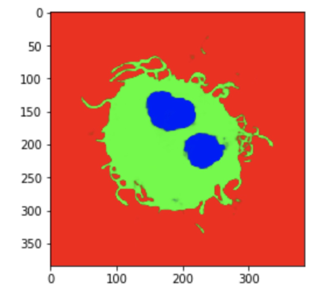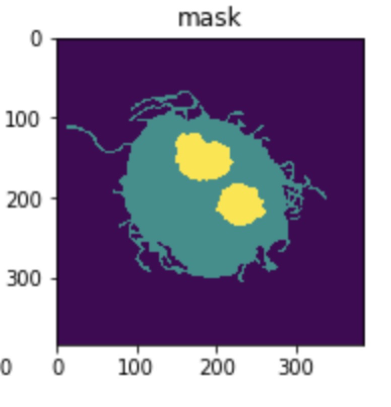MRI image QuickNAT overfitting

View codes on Github Feed one subject’s axial plane to QuickNAT, in total 182 images, batch size is 5, image size is 128 x 128, with 3,308,688 parameters, the loss could decrease to 0.11 with 500 epochs.

Compared to UNet, which needs 31,058,944 parameters to achieve 0.13 loss, QuickNAT is computational effective.

Training Strategy rethinking

For each subject, for one plane, e.g. axial plane, it has 182 slices. Whether to feed these 182 slices to the network every time, one subject by another subject, or feed all the slice in the same position to the network, i.e 330 slices per epoch, in total 182 epoch.
The experiments done before focus mainly on the first strategy, which turns out the loss doesn’t decrease significantly, though for one subject the loss may reach 0.5, but when training on a new subject, the first loss is 0.9 again. To my understand, that’s because for one subject, the 182 slices are different, so the weights are hard to generate. These two figures below illustrate the results:

QuickNAT with 3,308,688 parameters

Figure 2. One epoch every subject

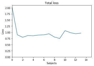
This figure above represents the loss where there is one iteration for each subject.

Fiture 3. 15 epochs every subject

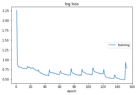
The figure 4 illustrate the loss where there are 15 epochs for each subject.

I will try the second strategy next week.

Paper Review

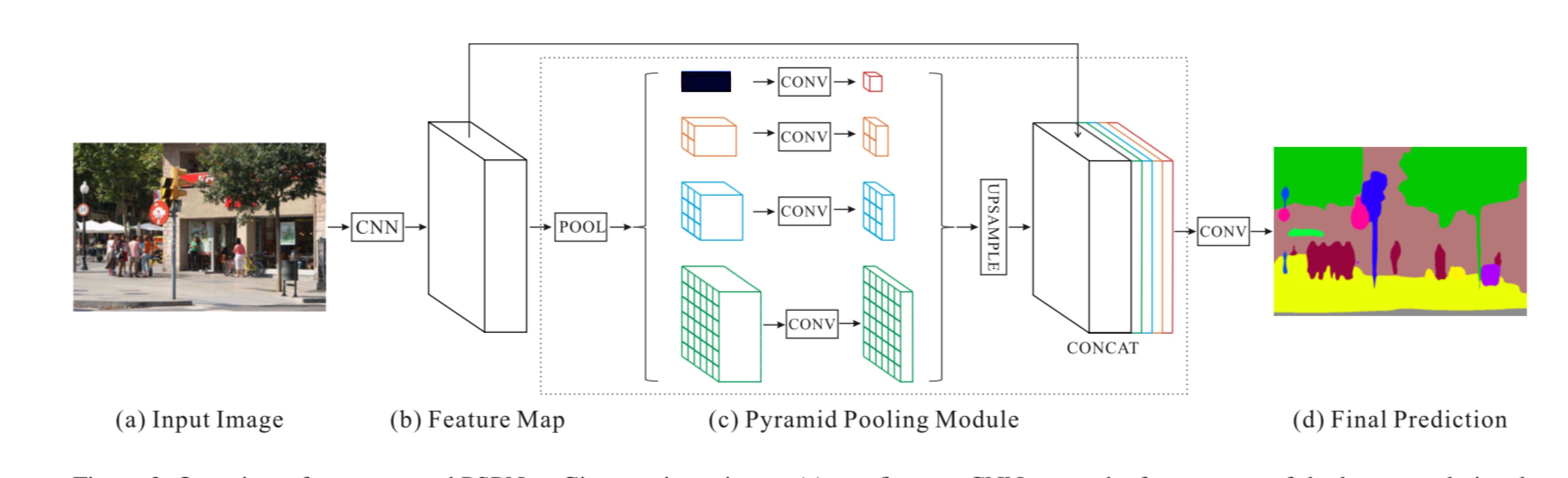
Zhao, Hengshuang, et al. “Pyramid Scene Parsing Network.” ArXiv:1612.01105 [Cs], Dec. 2016. arXiv.org. Link

1. Global context information <– different-region-based context aggregation <– pyramid pooling module
2. 85.4% on PASCAL VOL 2012, 80.2% on Cityscapes
3. Several problem under complex scene parsing:
   • Mismatched relationship –> Solution: add global context information
   • Confusion categories –> Solution: use relationship between different categories to identify categories
   • Inconspicuous class –> Solution: Pay more attention to different sub-regions that contain inconspicuous-category stuff.(QuickNAT add a weight parameter for each class)

Figure 4. PSP Network

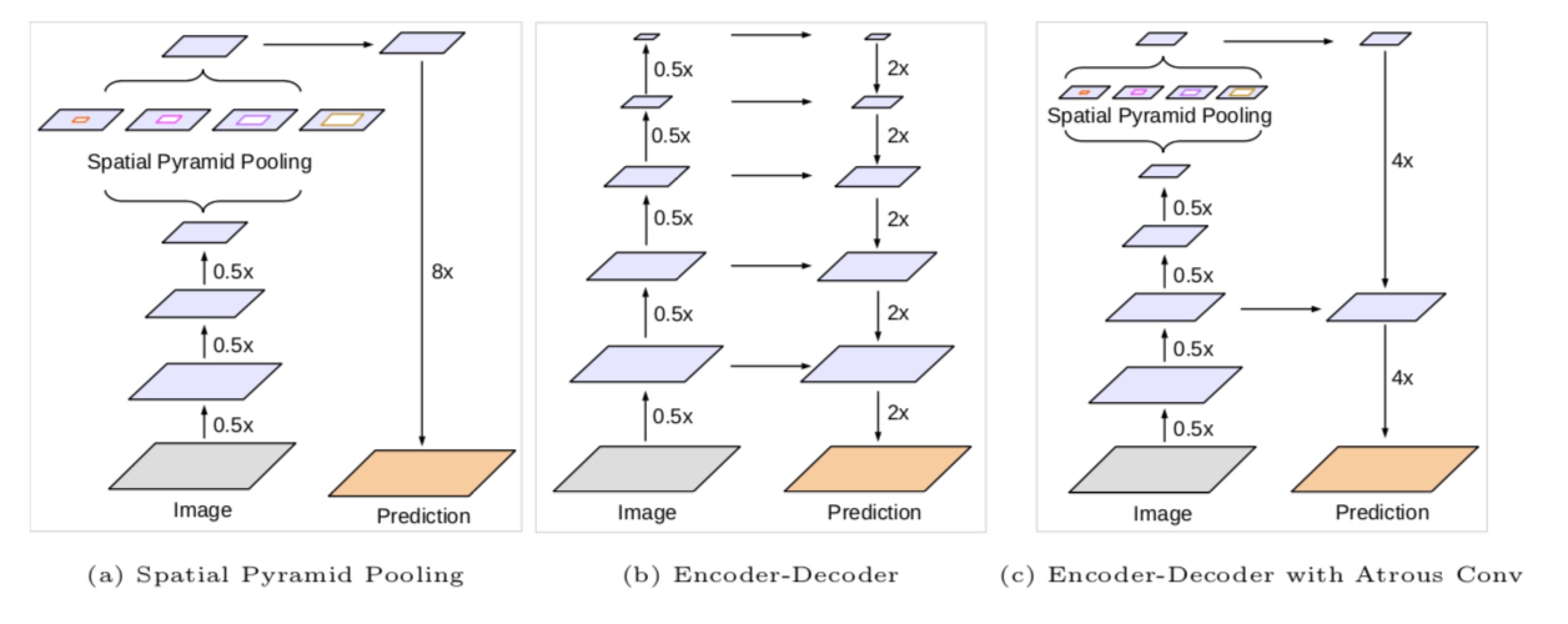
Chen, Liang-Chieh, et al. “Encoder-Decoder with Atrous Separable Convolution for Semantic Image Segmentation.” ArXiv:1802.02611 [Cs], Feb. 2018. arXiv.org. Link

Combine Encoder-decoder, pyramid scene parsing and atrous Convolution network together.

Figure 5. Encoder-decoder PSP Network

Luo, Wenjie, et al. “Understanding the Effective Receptive Field in Deep Convolutional Neural Networks.” ArXiv:1701.04128 [Cs], Jan. 2017. arXiv.org. Link

• For dense prediction, it is critical for each output pixel to have a big receptive field.
• Some pixels like the central ones will have their information propagated through many different paths in the network, while the pixels on the borders are propagated along a single path.

Figure 6. Receptive Field Illustration

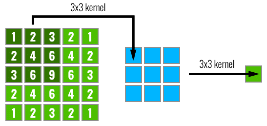
• The effective receptive field impact on the final output computation will look more like a Gaussian distribution.
• The effective area in the receptive field only occupies a fraction of the theoretical receptive field.
• This receptive field is dynamic and changes during training.
• As a result, the central pixels will have a larger gradient magnitude compared to the border pixels during backpropagation. related sources