Study Note of Course 4 - deeplearning.ai
12 Nov 2018- course source: deeplearning.ai
Week 1
Objectives: Understand Convolution operation Understand Pooling operation Remember Padding, Stride, filter,… Build Convolutional neural network for image multi-class classification
Computer Vision Problems
- Image Classaification
- Object Detection
- Neural Style Transfer
I. Padding
- Valid convolution: no padding
- Same convolution: Pad so that output size is the same as the input size
II. Summary of convolutions
- n x n image f x f filter
- padding p
- stride s
- output size: (n + 2p - f )/s + 1
III. MaxPooling and AveragePooling
- Hyperparameters:
- filter, normally : f=2
- stride, normally: s=2
- No parameters to learn
IV. Why convolutions
- Parameter sharing
- Sparsity of connections
Week 2
Objectives: Understand multiple foundational papers of CNN Analyze the dimensionality reduction of a volume in a very deep network Understand and Implement a Residual network Build a deep neural network using Keras Implement skip-connection Clone a repository from github and use transfer learning
I. Classic networks
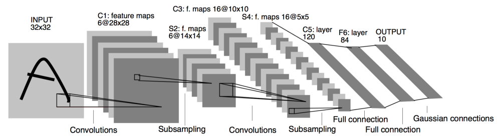
- LeNet-5_1998:
LeNet-5 Architecture
- Goal: Recognize handwritten digits
- Trained on grayscale images
- Input image (32x32x1) –> Conv (5x5 filter 6 filters s=1 no Padding) –> AveragePooling (f=2 s=2) –> Conv (16 filters 5x5 filter s=1) –> AveragePooling –> FC(120) –> FC (84) –> yhat (10 possible values)
- 60k parameters
- Go deeper in a network, the height and width tend to go down. Number of channels increase.
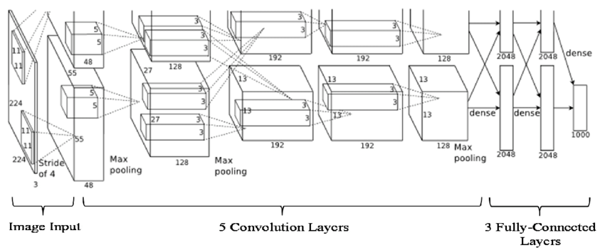
- AlexNet_2012: AlexNet Architecture
- Input image (227x227x3) —> Conv (11x11 filter 96 filters s=4) —> MAX-POOL (f=3 s=2) —> Cov (5x5 same padding) —> MAX-POOL (f=3 s=2) —> Conv (3x3 same padding) –> Conv (3x3 same padding) —> Conv (3x3 same padding) —> MAX-POOL (f=3 s=2) —> Unroll this into 9216 numbers —> 2 FC to 4096 nodes —> Softmax to output 1000
- Similarity to LeNet, but much bigger
- ~ 60 million parameters
- A lot more hidden units and train on a lot more data (ImageNet dataset), which enables remarkable performance.
- Use ReLu as the activation function
- Not used today:
- Multiple GPUs
- Local Response Normalization
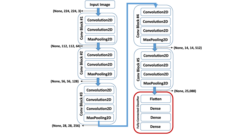
- VGG-16_2015: VGG-16 Architecture
- Much simpler network, a deep network
- All conv layers 3x3 filter s =1 same padding
- All max pool layers 2x2 s =2
- simplify the architecture
- 2 conv layers with 64 filters —> Pool layer —> 2 conv layers with 128 filters —> pool layer —> 3 conv layers with 256 filters —> Pool layer —> 3 conv layers with 512 filters —> pool layer —> 3 Conv Layers with 512 filters —> Pool Layer —> FC —> FC —> Softmax Output one of the 1000 classes. 1. ~138 million parameters
II. ResNet 152 layers
skip connections
- Enable the network to get deeper without harming the performance of the network. When the network gets deeper and deeper, it’s difficult to choose parameters to learn idendity function, while using the skip connections will solve this proble.
- Use the skip connections allows to add extra layers without hurting the performance of the network
- Skip connection also allows the gradient to be directly backpropagated to earlier layers. Residuel network
III. Inception 2014
- How to solve the problem of computational cost: add a 1x1 conv layer (bottleneck) to reduce the computational cost.
- The inception module do the convolution and max pooling in the same time and concatenate the result.
- Additional side branches: take some hidden layer to make some prediction. prevent overfitting
- You can use 1x1 Conv layer to reduce nc, but not nh, nw
- You can use pooling layer to reduce nh, nw, but not nc
IV. Transfer learning
Download weights that someone else has already trained on the network architecture and use that as pre-training. And transfer that to a new task that I might be interested in. Use it as an initial neural network.
- Download some open source implementation of a neural network, download not just the code but also the weights.
- If you have a very small training set, you can freeze all the parameters in the earlier layers and train only your own layer.
- If you have a larger training set, you can freeze some layers and train the other layers. Or add your own hidden layers.
- If you have a lot of data, you can take the open source network and weights, and use the whole thing just as initialization and train the whole network.
V. Data Augmentation
- Mirroring
- Random Cropping
- Rotation
- Shearing
-
Local warping
- Color shifting
PCA(AlexNet paper) color Augmentation
VI. Two sources of knowledge
- Labeled Data
- Hand engineered features/network architecture/other components For computer vision, there is not enough data, so it relys more on hand engineering.
VII. Doing well on benchmarks/winning competitions
- Ensembling (time consuming) – Train several networks independently and average their outputs. yhat.
- Multi-crop at test time (time consuming) – Run classifier on multiple versions of test images and average results
DO NOT USE IT FOR PRODUCT DEVELOPMENT IN THE REAL INDUSTRY
VIII. Use open source code
- use architectures of networks published in the literature
- use open source implementation if possible
- use pretrained models and fine-tune on your dataset
Week 3
Objectives: Understand the challenges of Object Localization, Object Detection and Landmark Finding Understand and implement non-max Suppression Understand and implement intersection over union Understand how we label a dataset for an object detection application Remember the vocabulary of object detection (landmark, anchor, bounding box, grid, …)
I. Object detection
- Classification with localization –> 1 big object
- Detection –> multiple objects
To locate the object, we output a bounding box: 4 parameters: bx, by, bh, bw
II. Landmark detection
Convolutional implementation of sliding windows detection algorithm, use only one forward pass to predict the output. More efficient
- YOLO algorithm
- Assign an object to a grid cell if the midpoint of the object is the grid cell.
- One object is assigned to only one grid cell.
- work very fast, even with the real time application
- By convention, the bounding box’s position is calculted relatively to the grid cell, the bx and by is between the 0 and 1. bh and bw could be larger than 1.
III. Intersection Over Union
- computes the size of the intersection over union of two bounding boxes of one object, divided by the size of the union.
- if IoU >= 0.5, it’s correct.
- The higher the IoU, the more accuracy the bounding box.
IV. Non-max Suppression
- A way to make sure that your algorithm detects each object only once. (one detection per object)
- Run object classification and localization algorithm for every one of these spilt cells
- Output the maximum probabilities classifications but suppress the close-by ones that are non-maximal
- Discard all boxes with p_c <= 0.6
- While there are any remaining boxes:
- Pick the box with the largest pc Output that as a prediction
- Discard any remaining box with IoU >= 0.5 with the box output in the previous step
V. Anchor boxes
- Each of the grid cell can only detect one object.
- In order to enable a grid cell to detect multiple objects, we introduce Anchor Boxes
- Pre-define 2 different shapes called, anchor boxes, associate two predictions with the two anchor boxes.
- Each object in training image is assigned to grid cell that contains object’s midpoint and anchor box for the grid cell with highest IoU.
VI. YOLO algorithm
- For each grid cell, get 2 predicted bounding boxes.
- Get rid of low probability predictions.
- For each class use non-max suppression to generate final predictions.
Week 4
Discover how CNNs can be applied to multiple fields, including art generation and face recognition. Implement your own algorithm to generate art and recognize faces!
Face Recognition
I. What is face recognition?
Face recognition & liveness detection
- Face verification
- Input image, name/ID
- Output whether the input image is that of the claimed person
- Face recognition
- Has a database of K persons
- Get an input image
- Output ID if the image is any of the K persons(or “not recognized”)
II. One Shot Learning
- For most face recognition applications, you need to be able to recognize a person given just one single image, or given just one example of that person’s face.
- Learn from just one example to recognize the person again
- The problem is the traning set is too small, using this training set to train a CNN will not give a robust network. Furthur, it’s hard to add person later, which requests retrain the network.
- To solve this problem, we will learn a similarity function: the network will learn a function inputs 2 images, outputs the degree of difference between the 2 images. If the 2 images are from the same person, we expect a small number as the output.
- During the recognition time, if the degree of difference between them is less than some threshold called τ, you could predict that these 2 pictures are the same person.
- If there is a new person join the team, just add it in the database, it works fine.
III. Siamese network_2014
- Feed the first image \(x_i\) to the CNN, get a vector of 128 numbers fxi.
- Feed the second image \(x_j\) to the same CNN with same parameters, get a different vector of 128 numbers.
- Define d() as the distance between the \(x_i\) and \(x_j\)
- The goal of learning: Learn parameters so that
- If \(x_i\) and \(x_j\) are the same person, \((fx_i - fx_j)^2\) is small.
- If \(x_i\) and \(x_j\) are different person, \((fx_i - fx_j)^2\) is large.
IV. Triplet Loss_2015
- Always look at one anchor image and you want the distance between the anchor and the positive image to be small, and the distance between the anchor and the negative image to be large.
- Always look at three images at a time.
- Want the encoding distance of \((f_a - f_p)^2\) to be smaller than \((f_a - f_n)^2\), i.e. \((f_a-f_p)^2 -(f_a -f_n)^2 <= \alpha\), α here is called margin.
- Loss function, given 3 images:
- \(L(A,P,N)=Max((f_a-f_p)^2 -(f_a -f_n)^2 + \alpha, 0)\)
- Overall cost function on your network : \(J = \displaystyle\sum_{i=1}^{m} L_i\)
- Tips:
- Choose triplets that’re “hard” to train on
V. Face Verification and Binary classification_2014
- Take this pair of Siamese networks and have them both compute these embeddings, and have these be input to a logistic regression unit to then just make a prediction.
- The target output will be one if both of these are the same persons, and zero if both of these are of different persons.
- Instead of having to compute the embedding every time adding a new person, you can pre-compute that. Use the upper Conv Net to compute the encoding and use it to compare it to your pre-computed encoding and then use that to make a prediction yhat.
- Compare to the triplet computation, this method compare 2 images one time, instead of 3 images.
Neural Style Transfer_ Gatys et al..2015
I. What are deep ConvNets learning?
- Pick a unit in layer 1. Find the nine image patches that maximize the unit’s activation. Repeat for other units.
- Define a Cost function
- Given a Content Image C and a Style image S, the goal is to generate a image G.
- In order to implement neural style transfer, we need to define a cost function J of G that mesures how good is a particular generated image and we’ll use gradient descent to minimize J(G) in order to generate this image.
- How good is this particular image? Define two parts to this cost function:
- Content cost function and the Style cost function.
- We weight these with two Hyperparameters α and β to specify the relative weighting between the content cost and the style cost.
- Find the generated image G
- Initiate G randomly
- Define the cost function J(G).
- Use gradient descend to minimize J(G).
II. Content Cost Function
- Overall Cost Function
- \[J(G) = \alpha J_c (C,G) + \beta J_s (S,G)\]
- Say you use hidden layer l to compute content cost
- Use pre-trained ConvNet.
- We want to know given a content image and a generated image, how similar is their content.
- If \(a_lC\) and \(a_lG\), the activation of layer l on the images are similar, both images have similar content.
III. Style Cost Function
- Say you are using layer l’s activation to mesure “style”.
- Define style as correlation between activations across channels.
- The correlation tells us which of these high level texture components tend to occur or not occur together.
- The correlation gives us one way of measuring how often these different high level features occur together in different